
views

Open your pivot table Excel document. Double-click the Excel document that contains your pivot table. It will open.

Go to the spreadsheet page that contains your data. Click the tab that contains your data (e.g., Sheet 2) at the bottom of the Excel window.
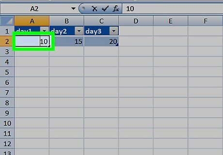
Add or change your data. Enter the data that you want to add to your pivot table directly next to or below the current data. For example, if you have data in cells A1 through E10, you would add another column in the F column or another row in the 11 row. If you simply want to change the data in your pivot table, alter the data here.

Go back to the pivot table tab. Click the tab on which your pivot table is listed.
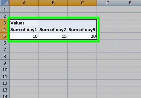
Select your pivot table. Click the pivot table to select it.

Click the Analyze tab. It's in the middle of the green ribbon that's at the top of the Excel window. Doing so will open a toolbar just below the green ribbon. On a Mac, click the PivotTable Analyze tab here instead.
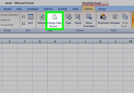
Click Change Data Source. This option is in the "Data" section of the Analyze toolbar. A drop-down menu will appear.

Click Change Data Source…. It's in the drop-down menu. Doing so opens a window.

Select your data. Click and drag from the top-left cell in your data group down to the bottom-left cell in the group. This will include the column(s) or row(s) that you added.
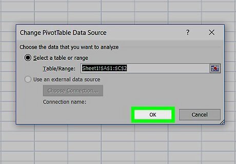
Click OK. It's at the bottom of the window.
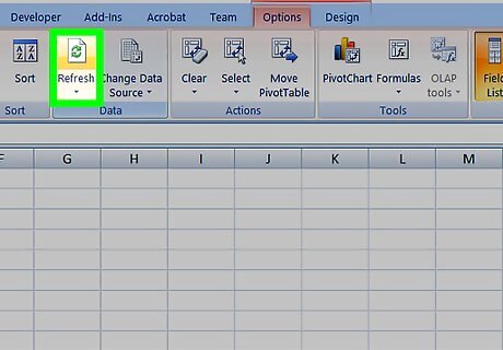
Click Refresh. It's in the "Data" section of the toolbar. If you added a new column to your pivot table, check its box in the right side of the Excel window to display it.


Comments
0 comment