views
Single Mode Function
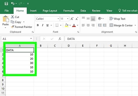
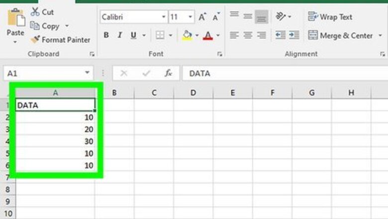
Enter each number in the data set into its own cell. If you’re looking for a single number that occurs most frequently in a group of numbers, use the MODE.SNGL function. For consistency, it helps to enter the number in consecutive cells in either a row or column, and for readability, a column is usually better. MODE.SNGL will only display one mode for a group of numbers. If your data has more than one mode (that is, multiple numbers that occur with equal frequency), this function will pick the first one in the set and ignore the others.
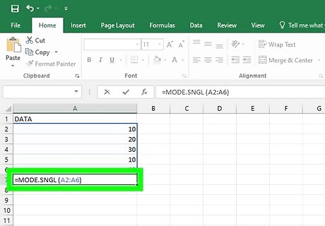
Enter the =MODE.SNGL function in the cell where you want the result. The MODE function's format is =MODE.SNGL(Cx:Dy), where C and D represent the letters of the columns of the first and last cell in the range, and x and y represent the numbers of the first and last row in the range. If all your data is in a single column, the 2 column letters will be the same (e.g., A1:A7). If you’re using a version of Excel older than 2010, write =MODE(Cx:Dy) without the .SNGL suffix. This will also work in the most recent versions of Excel. Either method will only return one mode result, even if there are multiple modes in the data set. You can also specify each cell individually, up to 255 cells, as in =MODE.SNGL(A1, A2, A3), but this can get cumbersome if you have a big dataset. You can also use the function with constants, for example, =MODE.SNGL(4,4,6), but this requires editing the function each time you wish to search for a different mode. You may want to format the cell in which the mode will display with bolding or italics to distinguish it from the numbers in the dataset, or put it in a separate column or row from the other numbers.
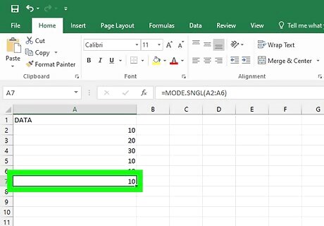
Calculate and display the result. This normally happens automatically in Excel, but if you have set up your spreadsheet for manual calculation, you'll need to press the F9 key to display the mode. Otherwise, as soon as you enter the formula and hit ↵ Enter, the mode should appear in the cell where you entered the function formula. For a dataset of 10, 7, 9, 8, 7, 0, and 4 entered in cells 1 through 8 of Column A, the function =MODE.SNGL(A1:A8) will deliver a result of 7, because 7 appears more often in the data than any other number. If the data set contains more than one number that qualifies as the mode (such as 7 and 9 each appearing twice and every other number appearing only once), whichever mode number is listed first in the data set will be the result. If none of the numbers in the data set appear more often than any other, the MODE function will display the error result #N/A. The MODE function will ignore any cells in the range that are blank or contain something other than a number.
Multiple Mode Function
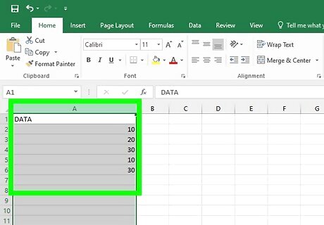
Enter each number in the data set into its own cell. The MODE.MULT function is useful if you have a dataset with more than one mode. To use it, first fill out a row or column with all the numbers in the set. The MODE.MULT function is only available in Excel 2010 and later versions. As an example of a data set with more than one mode, imagine that your group of numbers is 8, 7, 5, 7, 1, 3, and 8. 8 and 7 both appear twice in the group, and both are more frequent than any of the other numbers. These would be your modes.
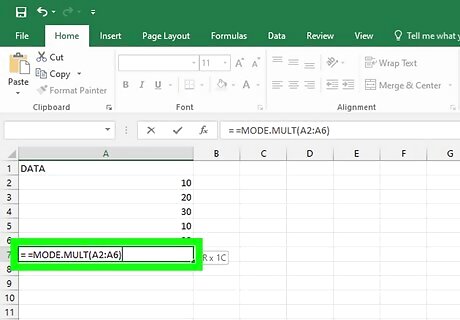
Enter the MODE.MULT function into the formula bar. The MODE.MULT function's format is =MODE.MULT(Cx:Dy), where C and D represent the first and last column letters in the range, and x and y are the row numbers of the first and last cells in the range. Select the cell where you want the first mode in the array to appear and type the formula into the formula bar or directly into the cell. For example, if your range includes the data in A1 through A29, you’d write =MODE.MULT(A1:A29). You can also type the individual cells or constants in the data set into the formula in place of the range, but this is only practical for very small data sets that you don’t plan to change. By default, this function will return all the modes for the selected range in the form of a vertical array—that is, it will create a column listing all the modes in the selected data range. If you’d rather view the modes as a horizontal array (that is, a row of results instead of a column), rewrite the formula as =TRANSPOSE(MODE.MULT(Cx:Dy)).
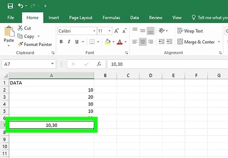
Hit ↵ Enter to display the modes. Once you type in the formula and hit ↵ Enter or ⏎ Return on your keyboard, the modes should automatically appear in an array starting with the selected cell. You might want to select a cell away from the rest of the data or use some type of special formatting (such as bold or italics) so you can tell the modes apart from the other numbers on the spreadsheet. If you’ve set the spreadsheet for manual calculations, hit F9 to calculate the modes. Otherwise, the array should update automatically any time you make changes to the data in the selected range. Just like MODE.SNGL, MODE.MULT will ignore any cells that are empty or contain data other than numbers. If there are no modes in the set—that is, if there’s no number that appears more times than any other in the group—you’ll get a result of #N/A.


Comments
0 comment