

Using the Tabular Method
Identify if the function you want to integrate can be solved by integrating by parts. If the function can be solved using integration by parts, it can also be solved by using tabular integration. For example, the function f ( x ) = x 2 c o s ( x ) {\displaystyle f(x)=x^{2}cos(x)} {\displaystyle f(x)=x^{2}cos(x)} can be solved by integrating by parts. Then, determine the substitutions for u {\displaystyle u} u and d v {\displaystyle \mathrm {d} v} {\mathrm {d}}v in the function. In this example, let u = x 2 {\displaystyle u=x^{2}} u=x^{2} and d v = c o s ( x ) d x {\displaystyle \mathrm {d} v=cos(x)\mathrm {d} x} {\displaystyle \mathrm {d} v=cos(x)\mathrm {d} x}.
Determine if you can use tabular integration to integrate the function. Repeatedly take the derivative of u {\displaystyle u} u. If you keep taking the derivative and it reaches 0 {\displaystyle 0} {\displaystyle 0}, then you can use tabular integration to find the antiderivative. For this example, when you take the first derivative of u = x 2 {\displaystyle u=x^{2}} u=x^{2}, you get 2 x {\displaystyle 2x} 2x, then the second derivative is 2 {\displaystyle 2} {\displaystyle 2}, and the third derivative is 0 {\displaystyle 0} {\displaystyle 0}, meaning that the tabular method will work with this example.
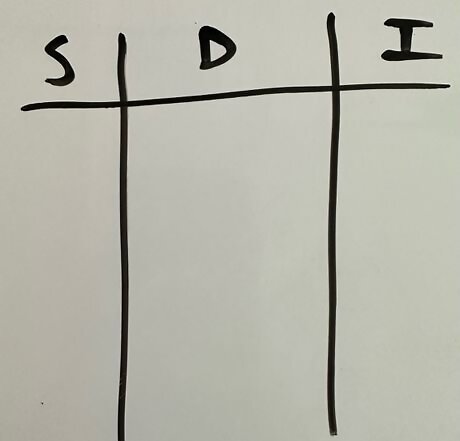
Create a table with three columns titled “S” for sign, “D” for derivative, and “I” for integral.
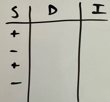
For the first row under “S”, write a positive/plus sign. In the second row, write a negative/minus sign. Alternate between positive/plus signs and negative/minus signs for each row.
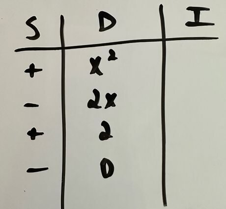
For the first row under “D”, write the substitution for u {\displaystyle u} u. For the second row, write the first derivative of u {\displaystyle u} u. For the third row, write the second derivative of u {\displaystyle u} u, or the derivative of the previous row. For the following rows, write the next derivative of the function based on the previous rows. Stop once the derivative results in 0 {\displaystyle 0} {\displaystyle 0}. For this example, write x 2 {\displaystyle x^{2}} x^{2} in the first row, then 2 x {\displaystyle 2x} 2x in the second row, then 2 {\displaystyle 2} {\displaystyle 2} in the third row, and 0 {\displaystyle 0} {\displaystyle 0} in the fourth and final row.
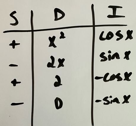
For the first row under “I”, write the substitution for d v {\displaystyle \mathrm {d} v} {\mathrm {d}}v, but omit the d x {\displaystyle \mathrm {d} x} {\mathrm {d}}x. For the second row, write the first antiderivative of d v {\displaystyle \mathrm {d} v} {\mathrm {d}}v. For the third row, write the second antiderivative of d v {\displaystyle \mathrm {d} v} {\mathrm {d}}v, or the antiderivative of the previous row. For the following rows, continue taking the antiderivatives. Stop when you reach the row where the “D” column stopped. For this example, write c o s ( x ) {\displaystyle cos(x)} {\displaystyle cos(x)} in the first row, then s i n ( x ) {\displaystyle sin(x)} sin(x) in the second row, then − c o s ( x ) {\displaystyle -cos(x)} {\displaystyle -cos(x)} in the third row, then − s i n ( x ) {\displaystyle -sin(x)} {\displaystyle -sin(x)} in the fourth and final row.
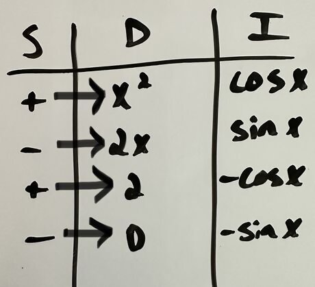
Multiply the sign from the “S” column by the derivatives from the “D” column for each row respectively. In this example, you will be left with x 2 {\displaystyle x^{2}} x^{2} in the first row, then − 2 x {\displaystyle -2x} -2x in the second row, then 2 {\displaystyle 2} {\displaystyle 2} in the third row, and 0 {\displaystyle 0} {\displaystyle 0} for the final row.
Multiply the derivatives in each row by the antiderivatives in the successive rows. In other words, multiply the derivative in the first row by the antiderivative in the second row, then multiply the derivative in the second row by the antiderivative in the third row, and so on until you reach the last row. For this example, you will end up with ( x 2 ) ( s i n ( x ) ) {\displaystyle (x^{2})(sin(x))} {\displaystyle (x^{2})(sin(x))} as the first term, then ( − 2 x ) ( − c o s ( x ) ) {\displaystyle (-2x)(-cos(x))} {\displaystyle (-2x)(-cos(x))} as the second term, then ( 2 ) ( − s i n ( x ) ) {\displaystyle (2)(-sin(x))} {\displaystyle (2)(-sin(x))} as the third and final term.
Simplify and combine the resulting terms to get the final antiderivative of the original function. Do not forget the + C {\displaystyle +C} +C! For this example, the antiderivative of f ( x ) = ( x 2 ) c o s ( x ) {\displaystyle f(x)=(x^{2})cos(x)} {\displaystyle f(x)=(x^{2})cos(x)} is ( x 2 ) s i n ( x ) + 2 x c o s ( x ) − 2 s i n ( x ) + C {\displaystyle (x^{2})sin(x)+2xcos(x)-2sin(x)+C} {\displaystyle (x^{2})sin(x)+2xcos(x)-2sin(x)+C}.
Deriving the Tabular Method: How it Works
Recall the formula for integration by parts. The formula is ∫ u d v = u v − ∫ v d u {\displaystyle \int u\mathrm {d} v=uv-\int v\mathrm {d} u} {\displaystyle \int u\mathrm {d} v=uv-\int v\mathrm {d} u}.
Consider the variables u {\displaystyle u} u and v {\displaystyle v} v as functions. Let u = f ( x ) {\displaystyle u=f(x)} {\displaystyle u=f(x)} and d v = g ( x ) d x {\displaystyle \mathrm {d} v=g(x)\mathrm {d} x} {\displaystyle \mathrm {d} v=g(x)\mathrm {d} x}, making d u = f ( 1 ) ( x ) {\displaystyle \mathrm {d} u=f^{(1)}(x)} {\displaystyle \mathrm {d} u=f^{(1)}(x)} (the first derivative of f {\displaystyle f} f) and v = g ( − 1 ) ( x ) {\displaystyle v=g^{(-1)}(x)} {\displaystyle v=g^{(-1)}(x)} (the first integral of g {\displaystyle g} g). Consider f {\displaystyle f} f as a polynomial function that, when you continuously take the derivative of it, you will end with 0 {\displaystyle 0} {\displaystyle 0}.
Substitute the variables back into the formula of integration by parts. You are left with ∫ f g d x = f g ( − 1 ) − ∫ f ( 1 ) g ( − 1 ) d x {\displaystyle \int fg\mathrm {d} x=fg^{(-1)}-\int f^{(1)}g^{(-1)}\mathrm {d} x} {\displaystyle \int fg\mathrm {d} x=fg^{(-1)}-\int f^{(1)}g^{(-1)}\mathrm {d} x}.
Use integration by parts again on the resulting integral, ∫ f ( 1 ) g ( − 1 ) d x {\displaystyle \int f^{(1)}g^{(-1)}\mathrm {d} x} {\displaystyle \int f^{(1)}g^{(-1)}\mathrm {d} x}. Doing so will result in the equation, ∫ f ( 1 ) g ( − 1 ) d x = f ( 1 ) g ( − 2 ) − ∫ f ( 2 ) g ( − 2 ) d x {\displaystyle \int f^{(1)}g^{(-1)}\mathrm {d} x=f^{(1)}g^{(-2)}-\int f^{(2)}g^{(-2)}\mathrm {d} x} {\displaystyle \int f^{(1)}g^{(-1)}\mathrm {d} x=f^{(1)}g^{(-2)}-\int f^{(2)}g^{(-2)}\mathrm {d} x}. By plugging this back into the original equation, you get ∫ f g d x = f g ( − 1 ) − ( f ( 1 ) g ( − 2 ) − ∫ f ( 2 ) g ( − 2 ) d x ) {\displaystyle \int fg\mathrm {d} x=fg^{(-1)}-\left(f^{(1)}g^{(-2)}-\int f^{(2)}g^{(-2)}\mathrm {d} x\right)} {\displaystyle \int fg\mathrm {d} x=fg^{(-1)}-\left(f^{(1)}g^{(-2)}-\int f^{(2)}g^{(-2)}\mathrm {d} x\right)}, which simplifies to ∫ f g d x = f g ( − 1 ) − f ( 1 ) g ( − 2 ) + ∫ f ( 2 ) g ( − 2 ) d x {\displaystyle \int fg\mathrm {d} x=fg^{(-1)}-f^{(1)}g^{(-2)}+\int f^{(2)}g^{(-2)}\mathrm {d} x} {\displaystyle \int fg\mathrm {d} x=fg^{(-1)}-f^{(1)}g^{(-2)}+\int f^{(2)}g^{(-2)}\mathrm {d} x}.
Continue to use integration by parts on the resulting integral until the derivative of f {\displaystyle f} f gives {\displaystyle 0} {\displaystyle 0} as the result. You will find a pattern, where the resulting integral gives f ( n − 1 ) g ( − ( n ) ) − ∫ f ( n ) g ( − ( n ) ) d x {\displaystyle f^{(n-1)}g^{(-(n))}-\int f^{(n)}g^{(-(n))}\mathrm {d} x} {\displaystyle f^{(n-1)}g^{(-(n))}-\int f^{(n)}g^{(-(n))}\mathrm {d} x}, where n {\displaystyle n} n represents how many times you used integration by parts. For this example, let's say that the fourth derivative f ( 4 ) {\displaystyle f^{(4)}} {\displaystyle f^{(4)}} is 0 {\displaystyle 0} {\displaystyle 0}. By plugging in and simplifying the original equation, you get ∫ f g d x = f g ( − 1 ) − f ( 1 ) g ( − 2 ) + f ( 2 ) g ( − 3 ) − f ( 3 ) g ( − 4 ) + C {\displaystyle \int fg\mathrm {d} x=fg^{(-1)}-f^{(1)}g^{(-2)}+f^{(2)}g^{(-3)}-f^{(3)}g^{(-4)}+C} {\displaystyle \int fg\mathrm {d} x=fg^{(-1)}-f^{(1)}g^{(-2)}+f^{(2)}g^{(-3)}-f^{(3)}g^{(-4)}+C} as the result, where each term alternatives in sign, or goes from plus to minus.
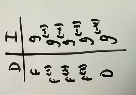
Make a table that organizes all of the derivatives of f {\displaystyle f} f under one column and the integrals of g {\displaystyle g} g in another column. Label the column for f {\displaystyle f} f as “D” and the column for g {\displaystyle g} g as “I”. Notice that each row corresponds to one of the resulting integrals from doing integration by parts.
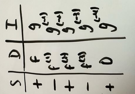
Create a new column for each alternating sign, and place it to the left of column “D”. Label this new column as “S”, and start with a plus sign, then minus sign, and keep alternating until you reach the last row.
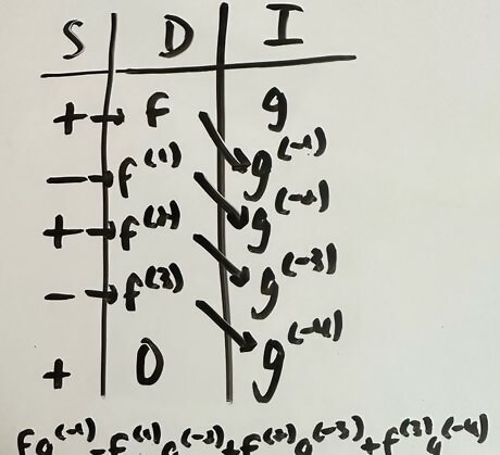
Notice that the derivatives in each row and the integrals in each successive row (ie. the derivative in the first row and the integral in the second row) match with the terms from the result of integrating by parts. Also, notice how the signs also match with the signs of the terms from integrating by parts. By writing out the result of the terms, notice that you end up with the same result as when you used integration by parts. From this example, it is clear that the tabular method is a quicker and cleaner way of doing integration by parts, but be careful, as it can only be used for certain problems, not all.


Comments
0 comment